Profiling
In the hls4ml configuration file, it is possible to specify the model Precision and ReuseFactor with fine granularity.
Using a low precision can help reduce the FPGA resource usage of a model, but may result in loss of model performance if chosen inappropriately. The profiling tools in hls4ml help you to decide the appropriate model precision.
Profiling uses some extra dependencies, to install these, run pip install hls4ml[profiling]. The profiling tools are provided as a Python module which you can use.
Three types of objects can be provided: a model object, test data, and a ModelGraph object. The model can be Keras or PyTorch.
You will need to initialise these objects by using a trained model, loading a model from a file, and loading your data. The Keras model and data each need to be in the format that would normally allow you to run, e.g. model.predict(X).
from hls4ml.model.profiling import numerical
from hls4ml.converters import keras_to_hls
import matplotlib.pyplot as plt
import yaml

# pseudo code:
model = load_model()
X = load_data()

# real code:
# load your hls4ml .yml config file with yaml
with open("keras-config.yml", 'r') as ymlfile:
    config = yaml.load(ymlfile)

hls_model = keras_to_hls(config)

# produce 4 plots
plots = numerical(model=model, hls_model = hls_model, X=X)
plt.show()
Calling the hls4ml.model.profiling.numerical method with these three objects provided will produce four figures as below:
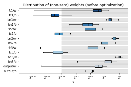
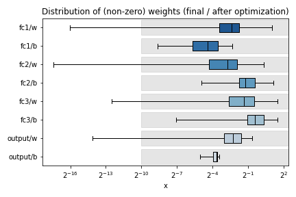
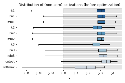
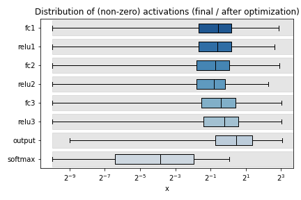
Plots are title “before optimization” and “final / after optimization”. The “before optimization” plots show the distributions of the original Keras or PyTorch model, while the “after optimization” plots show the distributions of the ModelGraph. In the example images, notice the “bn1”, “bn2”, “bn3” labels in the “before optimization” plots which are missing from the “after optimization”. These layer are BatchNormalization layers, which hls4ml has fused into the preceding Dense layers (labelled “fc{1,2,3}”). Because of this optimization, the weights of “fc1” of the ModelGraph are actually the product of the weights of the Keras model “fc1” with “bn1”. Similarly, the output of “fc1” of the ModelGraph should correspond to the output of the Keras model “bn1”. When optimizing precision, the data types should be chosen to work well for the “after optimization” model.
Different plots styles are available with the plot keyword argument. Valid options are boxplot (default), histogram, violinplot. In the default boxplot style, each variable in the neural network is evaluated using the given test data and the distribution of (non-zero) values is shown with a box and whisker diagram.
When different combinations of the input objects are given, different plots will be produced:
Only Keras or PyTorch model: only the weights profile plot will be produced, the activation profile will be
None. No grey boxes representing the data types will be shown.Only ModelGraph (or ModelGraph and Keras or PyTorch model): two weights profile plots will be produced, with grey boxes indicating the data types from the ModelGraph. The first plot is the “before optimization” model, while the second plot is the “after optimization” model.
Keras or PyTorch model and data (
X): both the weights profile and activation profile will be produced. No grey boxes representing the data types will be shown.Keras or PyTorch model, ModelGraph, and data: both weights and activation profiles are produced, with grey boxes indicating the data types from the ModelGraph.
Each box shows the median and quartiles of the distribution. The grey shaded boxes show the range which can be represented with the hls4ml config file used.
As a starting point, a good configuration would at least cover the box and whisker for each variable with the grey box. Make sure the box and whisker is contained to the right by using sufficient integer bits to avoid overflow. It might be that more precision is needed (grey boxes extend further to the left) to achieve satisfactory performance. In some cases, it is safe to barely cover the values and still achieve good accuracy.
To establish whether the configuration gives good performance, run C Simulation with test data and compare the results to your model evaluated on the CPU with floating point.